NBS pairwise tests
Lyron Winderbaum
2021-03-11
Last updated: 2021-05-17
Checks: 7 0
Knit directory: soybean_exploration/
This reproducible R Markdown analysis was created with workflowr (version 1.6.2). The Checks tab describes the reproducibility checks that were applied when the results were created. The Past versions tab lists the development history.
Great! Since the R Markdown file has been committed to the Git repository, you know the exact version of the code that produced these results.
Great job! The global environment was empty. Objects defined in the global environment can affect the analysis in your R Markdown file in unknown ways. For reproduciblity it’s best to always run the code in an empty environment.
The command set.seed(20210309) was run prior to running the code in the R Markdown file. Setting a seed ensures that any results that rely on randomness, e.g. subsampling or permutations, are reproducible.
Great job! Recording the operating system, R version, and package versions is critical for reproducibility.
Nice! There were no cached chunks for this analysis, so you can be confident that you successfully produced the results during this run.
Great job! Using relative paths to the files within your workflowr project makes it easier to run your code on other machines.
Great! You are using Git for version control. Tracking code development and connecting the code version to the results is critical for reproducibility.
The results in this page were generated with repository version 1459c97. See the Past versions tab to see a history of the changes made to the R Markdown and HTML files.
Note that you need to be careful to ensure that all relevant files for the analysis have been committed to Git prior to generating the results (you can use wflow_publish or wflow_git_commit). workflowr only checks the R Markdown file, but you know if there are other scripts or data files that it depends on. Below is the status of the Git repository when the results were generated:
Ignored files:
    Ignored:    .Rhistory
    Ignored:    .Rproj.user/

Untracked files:
    Untracked:  output/pairwise_tests_all_orig.csv
Note that any generated files, e.g. HTML, png, CSS, etc., are not included in this status report because it is ok for generated content to have uncommitted changes.
These are the previous versions of the repository in which changes were made to the R Markdown (analysis/NBS_pairwise_tests.Rmd) and HTML (docs/NBS_pairwise_tests.html) files. If you’ve configured a remote Git repository (see ?wflow_git_remote), click on the hyperlinks in the table below to view the files as they were in that past version.
| File | Version | Author | Date | Message |
|---|---|---|---|---|
| Rmd | 1459c97 | Lyron Winderbaum | 2021-05-17 | Fixed error in data caching and updated results to reflect fix |
| html | 6c7aa69 | Lyron Winderbaum | 2021-05-17 | Build site. |
| Rmd | b89d097 | Lyron Winderbaum | 2021-05-17 | Update discussion on NBS genes present in global interactions |
| Rmd | e17a079 | Lyron Winderbaum | 2021-05-17 | Pairwise Tests |
| html | e17a079 | Lyron Winderbaum | 2021-05-17 | Pairwise Tests |
# # Cleanup and Global Settings
# rm(list = ls())
# if (!is.null(sessionInfo()$otherPkgs)) {
#   invisible(lapply(paste0('package:', names(sessionInfo()$otherPkgs)),
#                    detach, character.only=TRUE, unload=TRUE))
# }
# graphics.off()
# options(stringsAsFactors = FALSE)

library(tidyverse)
── Attaching packages ──────────────────────────────────────────────────────────────────────── tidyverse 1.2.1 ──✔ ggplot2 3.2.1 ✔ purrr 0.3.2
✔ tibble 2.1.3 ✔ dplyr 0.8.3
✔ tidyr 1.0.0 ✔ stringr 1.4.0
✔ readr 1.3.1 ✔ forcats 0.4.0── Conflicts ─────────────────────────────────────────────────────────────────────────── tidyverse_conflicts() ──
✖ dplyr::filter() masks stats::filter()
✖ dplyr::lag() masks stats::lag()Read in and subset data
# Read tidy data saved at the of initial_data_organisation.Rmd
load(file.path('data', 'pav_data.RData'))

# Reduce to NBS genes
nbs_table = pav_table[, c(TRUE, names(pav_table)[-1] %in% nbs$Name)]

# Merge on Yield and reduce to lines for which we have yield data
meta.df = subset(meta.df, !is.na(Yield))
nbs_table = merge(meta.df[, c('Line', 'Yield')], nbs_table)

# Reduce to genes with some decent level of variation
nbs_table = nbs_table[, c(TRUE, TRUE, colMeans(nbs_table[, -(1:2)]) <= 0.98 & colMeans(nbs_table[, -(1:2)]) >= 0.02)]

# # Proportion presence
# hist(colMeans(nbs_table[, -(1:2)]))


# Simplify gene names slightly
names(nbs_table) = sub('00.1.p$', '', names(nbs_table))
names(nbs_table) = sub('^GlymaLee.', 'GL', names(nbs_table))
names(nbs_table) = sub('^UWASoyPan', 'UWA', names(nbs_table))

# Move Line information into row.names
row.names(nbs_table) = nbs_table$Line
nbs_table$Line = NULL
NBS Pairwise Tests
So, if we restrict to NBS genes that occur in at least 2% and no more than 98% of individuals in our dataset this leaves us with 76 genes (noting we shorten GlymaLee to GL and UWASoyPan to UWA for convenience):
gene_nms = names(nbs_table)[-1]
gene_nms
[1] "GL01G0309" "GL01G0884" "GL03G0420" "GL03G0421" "GL03G0454"
[6] "GL03G0455" "GL03G0456" "GL03G0457" "GL03G0459" "GL03G0706"
[11] "GL03G0707" "GL06G2286" "GL06G2289" "GL06G2291" "GL06G2293"
[16] "GL06G2305" "GL06G2306" "GL06G2326" "GL06G2328" "GL07G0600"
[21] "GL07G0702" "GL10G0346" "GL14G0220" "GL15G1986" "GL15G1992"
[26] "GL15G1993" "GL15G1995" "GL16G1111" "GL16G1113" "GL16G1115"
[31] "GL16G1308" "GL16G1752" "GL16G1755" "GL16G1756" "GL18G0757"
[36] "GL18G0763" "GL18G0766" "UWA00005" "UWA00022" "UWA00043"
[41] "UWA00155" "UWA00201" "UWA00202" "UWA00251" "UWA00276"
[46] "UWA00316" "UWA00326" "UWA00427" "UWA00670" "UWA00725"
[51] "UWA00772" "UWA00953" "UWA00975" "UWA01217" "UWA01253"
[56] "UWA01320" "UWA01330" "UWA01418" "UWA01530" "UWA01729"
[61] "UWA01876" "UWA01973" "UWA02043" "UWA02496" "UWA02799"
[66] "UWA03194" "UWA03230" "UWA03233" "UWA03261" "UWA03336"
[71] "UWA03340" "UWA03402" "UWA04314" "UWA04354" "UWA04967"
[76] "UWA05312" We we consider all possible pairwise interactions (of which there are 2850), and perform a t-test for the interaction term in these linear models with Yield as the response:
gene_nms = names(nbs_table)[-1]
df_pairs = data.frame()
for (i in 1:(length(gene_nms)-1)) {
  for (j in (i + 1):length(gene_nms)) {
    f = as.formula(paste('Yield ~', gene_nms[i], '*', gene_nms[j]))
    m = lm(f, data = nbs_table)
    int_nm = paste0(gene_nms[i], ':', gene_nms[j])
    if (int_nm %in% row.names(summary(m)$coefficients)) {
      df_pairs = rbind(
        df_pairs,
        data.frame(gene.1 = gene_nms[i], gene.2 = gene_nms[j],
                   p.val = summary(m)$coefficients[int_nm, "Pr(>|t|)"])
      )
    } else {
       df_pairs = rbind(
        df_pairs,
        data.frame(gene.1 = gene_nms[i], gene.2 = gene_nms[j], p.val = NA)
      )
    }
  }
}

df_pairs = df_pairs[order(df_pairs$p.val),]
df_pairs = na.omit(df_pairs)
234 of these interactions cannot be computed (because there is no difference in gene presence/absence between the genes), leaving us with 2764 interactions. Lets have a quick look at the p-value distribution:
hist(df_pairs$p.val)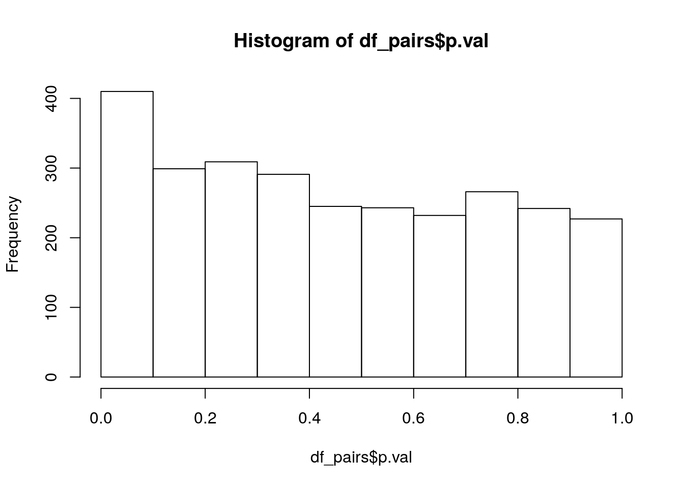
| Version | Author | Date |
|---|---|---|
| e17a079 | Lyron Winderbaum | 2021-05-17 |
sig_lvl = c(0.1, 0.05, 0.01)
rbind(sig_lvl,
      p_vals = sapply(sig_lvl, function(x){return(sum(df_pairs$p.val < x))}))
[,1] [,2] [,3]
sig_lvl 0.1 0.05 0.01
p_vals 410.0 234.00 83.00But we should apply a correction for multiple testing, using the Holm-Bonferroni method we get:
sig_lvl = c(0.1, 0.05, 0.01)
rbind(sig_lvl,
      p_vals = sapply(sig_lvl, function(x){return(sum(df_pairs$p.val*(nrow(df_pairs):1) < x))}))
[,1] [,2] [,3]
sig_lvl 0.1 0.05 0.01
p_vals 3.0 3.00 1.00So which are these three interesting interactions?
subset(df_pairs, p.val*(nrow(df_pairs):1) < 0.05) gene.1 gene.2 p.val
2524 UWA00725 UWA04967 3.520042e-06
1006 GL06G2293 UWA01973 4.094386e-06
2240 UWA00155 UWA01876 1.020067e-05Global Pairwise Tests
We can try the same procedure for all genes, not just the NBS genes. But first lets just tidy the full data in the same way we tidied the NBS data.
pav_table = merge(meta.df[, c('Line', 'Yield')], pav_table)

# Reduce to genes with some decent level of variation
pav_table = pav_table[, c(TRUE, TRUE, colMeans(pav_table[, -(1:2)]) <= 0.98 & colMeans(pav_table[, -(1:2)]) >= 0.02)]
The filter to only include genes with proportion of occurance between 2% and 98% reduces the 51415 genes down to just 2648 genes — a huge number of these genes are either very rare or very common, making it difficult to assess their imporance on Yield to to sample size limitations. Finish tidying:
# Simplify gene names slightly
names(pav_table) = sub('00.1.p$', '', names(pav_table))
names(pav_table) = sub('^GlymaLee.', 'GL', names(pav_table))
names(pav_table) = sub('^UWASoyPan', 'UWA', names(pav_table))

# Move Line information into row.names
row.names(pav_table) = pav_table$Line
pav_table$Line = NULL
and we can repeat the pairwise test procedure:
gene_nms = names(pav_table)[-1]
# source(file.path('analysis', 'pairwise_tests_all.R'))
df_pairs = read.csv(file.path('output', 'pairwise_tests_all.csv'))
df_pairs$gene.1 = gene_nms[df_pairs$gene.1]
df_pairs$gene.2 = gene_nms[df_pairs$gene.2]

df_pairs = df_pairs[order(df_pairs$p.val),]
df_pairs = na.omit(df_pairs)
Note I did some hackery there to run the code in a seperate script, store output, and load it in a particular format to get around re-running slow clode and get around the GitHub file size limit.
Of the 3,499,335 pairs of genes, 373,817 cannot compute interaction terms because of the two genes having exact overlap. This leaves 3,125,518 pairs for testing. Lets take a look at the p-value distribution:
hist(df_pairs$p.val)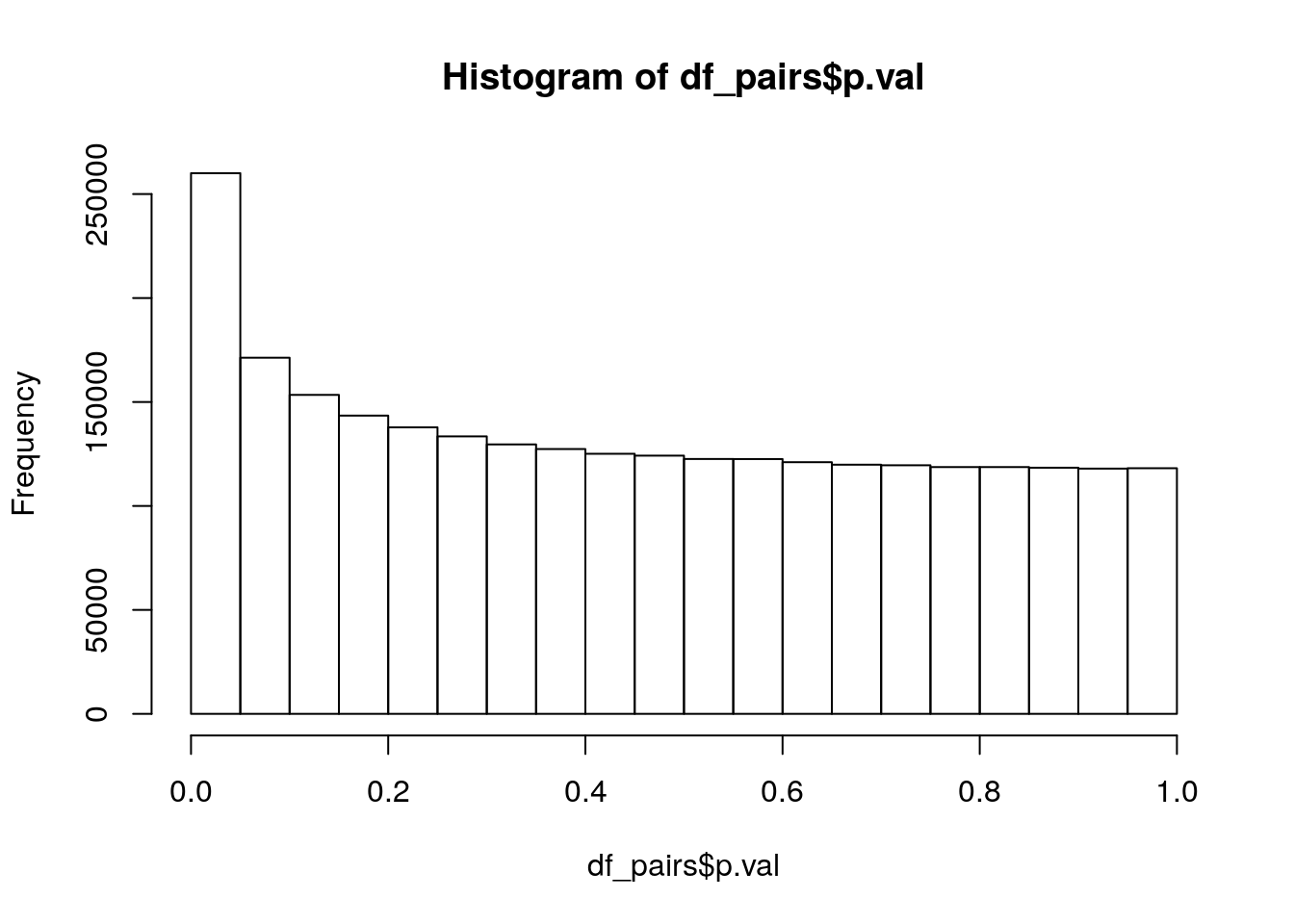
| Version | Author | Date |
|---|---|---|
| e17a079 | Lyron Winderbaum | 2021-05-17 |
Nice, lookes like a clear addition between a uniform distribution and an exponential distribution, just what we would expect if there are some real interactions mixed in. Lets count the small p-values:
sig_lvl = c(0.1, 0.05, 0.01)
rbind(sig_lvl,
      p_vals = sapply(sig_lvl, function(x){return(sum(df_pairs$p.val < x))}))
[,1] [,2] [,3]
sig_lvl 0.1 0.05 0.01
p_vals 431342.0 260053.00 85290.00and adjust for multiple testing using the Holm-Bonferroni method:
sig_lvl = c(0.1, 0.05, 0.01)
rbind(sig_lvl,
      p_vals = sapply(sig_lvl, function(x){return(sum(df_pairs$p.val*(nrow(df_pairs):1) < x))}))
[,1] [,2] [,3]
sig_lvl 0.1 0.05 0.01
p_vals 111.0 79.00 38.00So which are these 38 interesting interactions significant at the 1% level after multiple test correction?
subset(df_pairs, p.val*(nrow(df_pairs):1) < 0.01) gene.1 gene.2 p.val
1346684 UWA00331 UWA03376 1.102856e-13
1141561 UWA00124 UWA05001 1.958727e-13
2451105 UWA01903 UWA02125 6.146775e-13
1193847 UWA00183 UWA00331 6.363480e-13
1649641 UWA00731 UWA04571 2.944997e-12
2552295 UWA02183 UWA04253 2.986282e-12
1580983 UWA00627 UWA00884 4.987603e-12
2525414 UWA02125 UWA03239 1.142622e-11
1346205 UWA00331 UWA02131 1.343754e-11
1260127 UWA00245 UWA02125 1.408472e-11
1100273 UWA00078 UWA01330 1.810912e-11
795203 GL16G1461 UWA00222 7.721450e-11
1046103 UWA00005 UWA00331 9.987116e-11
2785774 UWA05056 UWA05133 1.664597e-10
798428 GL16G1462 UWA02466 2.077257e-10
796434 GL16G1461 UWA02466 2.603432e-10
2061196 UWA01259 UWA02319 2.879676e-10
1923840 UWA01081 UWA01910 2.956599e-10
1841404 UWA00988 UWA01064 3.966186e-10
2126279 UWA01381 UWA03673 5.026466e-10
2023626 UWA01210 UWA03078 6.680222e-10
103727 GL03G0274 UWA00771 6.977990e-10
2497372 UWA02062 UWA03639 7.710352e-10
797197 GL16G1462 UWA00222 7.871351e-10
723312 GL15G1995 UWA01260 9.280403e-10
722857 GL15G1995 UWA00411 9.899005e-10
1055830 UWA00014 UWA01135 1.267221e-09
1143517 UWA00126 UWA00331 1.676407e-09
785873 GL16G1403 UWA01438 1.959441e-09
1064550 UWA00023 UWA00045 2.090802e-09
1924575 UWA01081 UWA04457 2.398337e-09
2770651 UWA03673 UWA04229 2.679098e-09
1088998 UWA00054 UWA00884 2.826983e-09
562540 GL12G1178 UWA02412 3.051131e-09
1176847 UWA00163 UWA01910 3.115504e-09
1346778 UWA00331 UWA03891 3.330527e-09
785386 GL16G1403 UWA00543 3.414061e-09
1099677 UWA00078 UWA00202 3.562766e-09Do any of these interactions involve NBS genes? Yes! UWA00005, GL15G1995, UWA01330, and UWA00202. Are any of these interactions between NBS genes? No! they are all pairs of one NBS gene to one non-NBS gene:
subset(df_pairs, p.val*(nrow(df_pairs):1) < 0.01 & (gene.1 %in% names(nbs_table)[-1] | gene.2 %in% names(nbs_table)[-1])) gene.1 gene.2 p.val
1100273 UWA00078 UWA01330 1.810912e-11
1046103 UWA00005 UWA00331 9.987116e-11
723312 GL15G1995 UWA01260 9.280403e-10
722857 GL15G1995 UWA00411 9.899005e-10
1099677 UWA00078 UWA00202 3.562766e-09
sessionInfo()R version 3.6.3 (2020-02-29)
Platform: x86_64-pc-linux-gnu (64-bit)
Running under: Ubuntu 18.04.5 LTS
Matrix products: default
BLAS: /usr/lib/x86_64-linux-gnu/openblas/libblas.so.3
LAPACK: /usr/lib/x86_64-linux-gnu/libopenblasp-r0.2.20.so
locale:
[1] LC_CTYPE=en_AU.UTF-8 LC_NUMERIC=C
[3] LC_TIME=en_AU.UTF-8 LC_COLLATE=en_AU.UTF-8
[5] LC_MONETARY=en_AU.UTF-8 LC_MESSAGES=en_AU.UTF-8
[7] LC_PAPER=en_AU.UTF-8 LC_NAME=C
[9] LC_ADDRESS=C LC_TELEPHONE=C
[11] LC_MEASUREMENT=en_AU.UTF-8 LC_IDENTIFICATION=C
attached base packages:
[1] stats graphics grDevices utils datasets methods base
other attached packages:
[1] forcats_0.4.0 stringr_1.4.0 dplyr_0.8.3 purrr_0.3.2
[5] readr_1.3.1 tidyr_1.0.0 tibble_2.1.3 ggplot2_3.2.1
[9] tidyverse_1.2.1
loaded via a namespace (and not attached):
[1] tidyselect_1.1.0 xfun_0.10 haven_2.3.1 lattice_0.20-41
[5] colorspace_1.4-1 vctrs_0.3.1 generics_0.0.2 htmltools_0.4.0
[9] yaml_2.2.0 rlang_0.4.6 later_1.0.0 pillar_1.4.2
[13] withr_2.1.2 glue_1.3.1 modelr_0.1.5 readxl_1.3.1
[17] lifecycle_0.1.0 munsell_0.5.0 gtable_0.3.0 workflowr_1.6.2
[21] cellranger_1.1.0 rvest_0.3.4 evaluate_0.14 knitr_1.25
[25] httpuv_1.5.2 broom_0.5.2 Rcpp_1.0.3 promises_1.1.0
[29] backports_1.1.5 scales_1.0.0 jsonlite_1.6 fs_1.3.1
[33] hms_0.5.1 digest_0.6.23 stringi_1.4.3 grid_3.6.3
[37] rprojroot_1.3-2 cli_1.1.0 tools_3.6.3 magrittr_1.5
[41] lazyeval_0.2.2 crayon_1.3.4 whisker_0.4 pkgconfig_2.0.3
[45] xml2_1.2.2 lubridate_1.7.4 assertthat_0.2.1 rmarkdown_1.16
[49] httr_1.4.1 rstudioapi_0.10 R6_2.4.0 nlme_3.1-149
[53] git2r_0.26.1 compiler_3.6.3